LSTM (Long Short-Term Memory) models is a type of recurrent neural network (RNN). Recurrent neural networks use the output of the previous layer as the input, and they can retain information about previous time steps in the sequence.
This works really well for time series because we are taking into account previous layers, and therefore, the time aspect of the data, its history.

Retrieving Data

We have a stock market dataset that contains values from 2010 to 2019. The training dataset contains the values from 2010 to 2018. And the testing dataset contains values from 2018 to 2019. The features are the following : Date, Open, High, Low, Close, Adj Close, Volume.
We are only interested here in the Open values.
The training dataset and the testing dataset are in separate csv files. We will use pandas to read the csv files.

(Link to get the two csv files)

import pandas as pd
data_train = pd.read_csv('training_data.csv')
data_test = pd.read_csv('test_data.csv')

data_train    

    	  Date	         Open	           High	         Low            Close          Adj Close	   Volume
0	2010-07-28	37.667141	37.998573	37.178570	37.279999	32.658363	129996300
1	2010-07-29	37.244286	37.521427	36.585712	36.872856	32.301701	160951700
2	2010-07-30	36.555714	37.099998	36.414288	36.750000	32.194061	112052500
3	2010-08-02	37.205715	37.512856	37.088570	37.407143	32.769741	107013900
4	2010-08-03	37.287144	37.608570	37.060001	37.418571	32.779743	104413400

This is head of the training dataset.

Data Preparation

We are going to be retrieving the second column of the training dataset and the testing dataset.

data_train = data_train.iloc[:,1:2].values
data_test = data_test.iloc[:,1:2].values

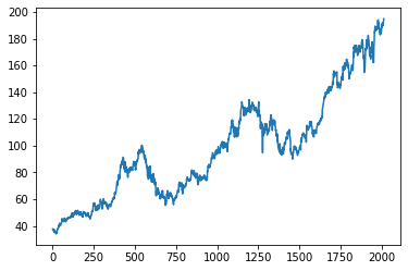
Let's visualize data_train.

import matplotlib.pyplot as plt
plt.plot(data_train)

This is what data_train looks like. We can see that we have some trend and seasonality in the dataset.

For data preparation, we are going to start by scaling our data. This is very important for time series to capture data properly at different time scales. We are making sure that each observation is treated equally.

We will be using MinMaxScaler from scikit-learn library. If we don't specify the range of the scale, then by default the range will be (0,1).

from sklearn.preprocessing import MinMaxScaler
scaler = MinMaxScaler()
scaler.fit(data_train)
data_train_scaled = scaler.transform(data_train)
data_test_scaled = scaler.transform(data_test)

data_train_scaled                

array([[0.022744  ],
       [0.02011732],
       [0.01584005],
       ...,
       [0.98801121],
       [0.9976395 ],
       [1.        ]])

For the final and most important step, we will be creating samples, reshaping our dataset and creating x_train, y_train from data_train and x_test, y_test from data_test.
The idea behind this is to make the data into the following format :

# Let's say this is our data
data_train = [ [10], [7], [35], [20], [9], [2], [17], [85] , ... ]
t_step = 3

# Creating x_train, y_train from data_train with a "sliding windows", t_step=3
x_train = [ [[10], [7], [35]], [[7], [35], [20]], [[35], [20], [9]], [[20],[9],[2]],
            [[9],[2],[17]] ... ]
y_train = [ [20], [9], [2], [17], [85] ... ]

What is above is just an example. Our data will not be looking like that because, remember, we have scaled it.
But this is the transformation that we are doing to be doing to our datasets.

For train_data

m_train, n_train = data_train.shape
m_test, n_test = data_test.shape

t_step = 60
y_train = list()
x_train = list()

for i in range(t_step,m_train):
  # Create temporary samples
  sample_x_train = data_train_scaled[i-t_step:i]
  sample_y_train = data_train_scaled[i]


  # Let’s add a padding
  if sample_x_train.shape[0] < t_step:
    var = np.zeros((t_step - sample_x_train.shape[0]),1)
    sample_x_train = np.concatenate((sample_x_train, var), axis = 0)
    sample_y_train = np.concatenate((sample_y_train, var), axis = 0)


  # Adding to the lists x_train, y_train
  x_train.append(sample_x_train)
  y_train.append(sample_y_train)

x_train = np.array(x_train)
y_train = np.array(y_train)

For test_data

t_step = 60
y_test = list()
x_test = list()

for i in range(t_step,m_test):
  # Create temporary samples
  sample_x_test = data_test_scaled[i-t_step:i]
  sample_y_test = data_test_scaled[i]


  # Let’s add a padding
  if sample_x_test.shape[0] < t_step:
    var = np.zeros((t_step - sample_x_test.shape[0]),1)
    sample_x_test = np.concatenate((sample_x_test, var), axis = 0)
    sample_y_test = np.concatenate((sample_y_test, var), axis = 0)


  # Adding to the lists x_test, y_test
  x_test.append(sample_x_test)
  y_test.append(sample_y_test)



x_test = np.array(x_test)
y_test = np.array(y_test)

Now that our data is preprocessed, let's create the LSTM model!

LSTM model

model = Sequential()
model.add(LSTM(units = 50, activation = "tanh", return_sequences = True, batch_size
= (None, t_step, 1))) #output 50
model.add(Dropout(0.1))  #dropout rate of 0.1
model.add(LSTM(units = 50, activation = "tanh", return_sequences = False))
model.add(Dropout(0.1))
model.add(Dense(units = 1)) #output layer

model.compile(loss='mse', optimizer='adam')
model.fit(x_train, y_train, epochs=100)
model.evaluate(x_test, y_test)

Our model has been created! You can play around with these parameters to decrease the loss of the model and reduce errors between y_test and y_pred. To predict y_test, we can use :

y_pred = model.predict(y_test)

And for the errors between y_test and y_pred :

import tensorflow as tf

tf.keras.metrics.mean_squared_error(y_test, y_pred)

Results

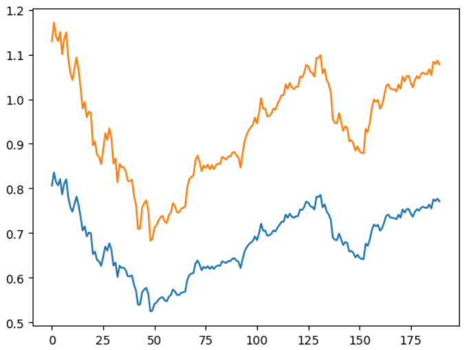
We can plot the results so that we can notice the difference between the predictions and the real value

plt.plot(y_test)
plt.plot(y_pred)

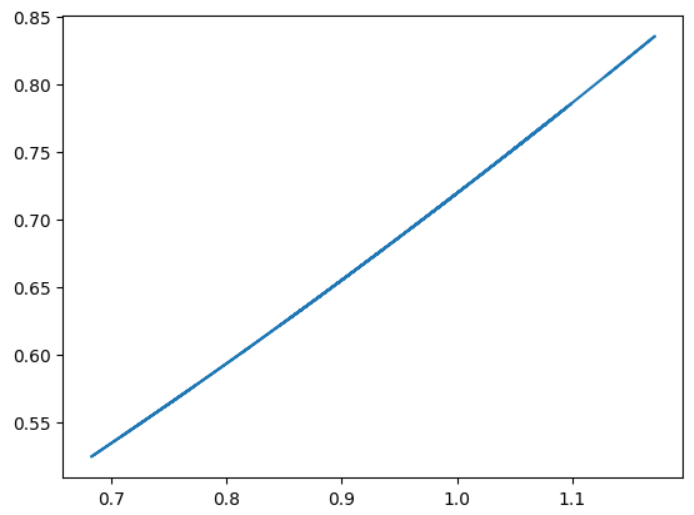
plt.plot(y_test,y_pred)

The results are really not that bad. The model is able to capture important patterns and relationships in the data, like the trend and the seasonality. And it is very much close to the real values as we can see.
As for the second plot, the idea is to simply to plot it as x=y and to see the linearity if it exists and in this case it kind of does!
We can also try to There may still be room for improvement for this model, but we will stick with this for now.

If you have any questions or wants to know more about the project, feel free to email me or tweet at me!

Related : Introduction To Machine Learning

---

Join my newsletter for similar articles and early access